Formatting Sandbox II: please *don't* test stuff here [duplicate]

Question

This thread has been retired due to the large number of posts. The newest sandbox can be found here:

Formatting Sandbox III: please test stuff here

Spoiler warning: Be aware that this page contains a lot of MathJax, so it will probably need quite a while to load completely.

User of the old sandbox will have noticed that with the amount of answers gathered there, it is very hard on your computer to get past the posts to the answer field. (Even deleting answers would not solve this problem for 10k users.)

Here you have a new playground... have fun.
(Use this for testing stuff instead of bumping random posts to the mainspace a million times.)

Before you delete a post here, please reduce it to one line without MathJax.

---

Old formatting sandboxes:

• Formatting Sandbox I: please test stuff here

Answer 1

So long and thanks for all the fish!

Answer 2

Wrong space around stretchy parentheses

$$\begin{align} y&=a\cdot b/(c\cdot d)\tag{ok}\\[6pt] y&=a\cdot b/\left(c\cdot d\right)\tag{?!}\\[6pt] y&=a\cdot b/{\left(c\cdot d\right)}\tag{ok}\\[6pt] y&=a\cdot b/\mathord{\left(c\cdot d\right)}\tag{ok} \end{align}$$

$$\begin{align} y&=\sum\limits_{i = 1}^n a_i\cdot b_i/(c_i^2\cdot d_i^2)\tag{ok}\\[6pt] y&=\sum\limits_{i = 1}^n a_i\cdot b_i/\left(c_i^2\cdot d_i^2\right)\tag{?!}\\[6pt] y&=\sum\limits_{i = 1}^n a_i\cdot b_i/{\left(c_i^2\cdot d_i^2\right)}\tag{ok}\\[6pt] y&=\sum\limits_{i = 1}^n a_i\cdot b_i/\mathord{\left(c_i^2\cdot d_i^2\right)}\tag{ok} \end{align}$$

$$\begin{align} f(x)&=x^2\tag{ok}\\[6pt] f\left(x\right)&=x^2\tag{?!}\\[6pt] f{\left(x\right)}&=x^2\tag{ok}\\[6pt] f\mathord{\left(x\right)}&=x^2\tag{ok} \end{align}$$

$$\begin{align} y&=\log(x)\tag{?}\\[6pt] y&=\log\left(x\right)\tag{?}\\[6pt] y&=\log{\left(x\right)}\tag{?}\\[6pt] y&=\log\mathord{\left(x\right)}\tag{?} \end{align}$$

Answer 3

Decision threshold and detection limit

General aspects

$$\textbf{Quantities and symbols}\\ \begin{array}{ll} \hline \text{Symbol}&\text{Name}\\ \hline y&\text{Estimate of the measurand}\\[-3pt] &\text{(e.g. measurement result of the measurand)}\\ u{\left(y\right)}&\text{Standard uncertainty of the measurand}\\[-3pt] &\text{(associated with the measurement result }y)\\ \tilde y&\text{True value of the measurand }\\ \tilde u{\left(\tilde y\right)}&\text{Standard uncertainty of an estimator of the measurand}\\[-3pt] &\text{(as a function of the true value of the measurand }\tilde y)\\ y^*&\text{Decision threshold}\\ y^\#&\text{Detection limit}\\ \hline x&\text{Estimate of the input quantity}\\ \hline \alpha&\text{Probability of the error of the first kind}\\ \beta&\text{Probability of the error of the second kind}\\ k_{1-\alpha}&\text{Quantile of the standardized normal distribution for the probability }\alpha\\ k_{1-\beta}&\text{Quantile of the standardized normal distribution for the probability }\beta\\ \hline \end{array}$$

In general, the result of a measurement $y$ is only an approximation or estimate of the value of the measurand and thus is complete only when accompanied by a statement of the uncertainty $u{\left(y\right)}$ of that estimate. Nevertheless, it is understood that the result of the measurement $y$ is the best estimate of the value of the measurand. The alternative best estimate $\hat y$, which explicitly takes into account the fact that the measurand is non-negative according to ISO 11929 and which differs from the measurement result $y$, is not used in the following examples.

For the provision and numerical calculation of the decision threshold $y^*$ and of the detection limit $y^\#$, the standard uncertainty $\tilde u$ of the measurand is needed as a function $\tilde u{\left(\tilde y\right)}$ of the true value $\tilde y$ of the measurand. This function is be determined in a way similar to $u{\left(y\right)}$ in accordance with ISO/IEC Guide 98-3. Usually, $\tilde u{\left(\tilde y\right)}$ can be explicitly specified, provided that $\tilde u{\left(\tilde y\right)}$ is given as a function of the primary measurement result $x$, which is taken as input quantity in the model of the evaluation $y{\left(x\right)}$ for the calculation of $y$. In this case, $y$ is be formally replaced by $\tilde y$ and the equation for $y{\left(x\right)}$ is solved for $x$. The result replaces $x$ in the equation of $u{\left(y\right)}$, which finally yields $\tilde u{\left(\tilde y\right)}$.

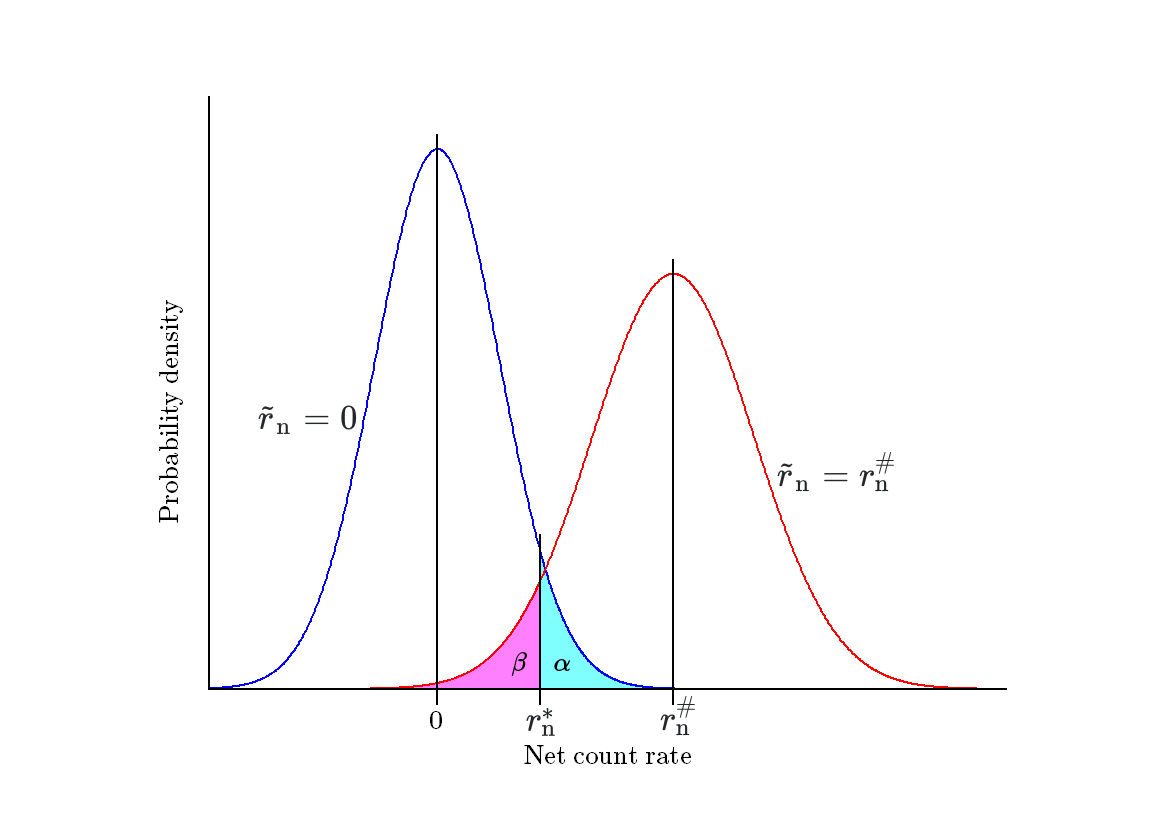
The decision threshold $y^*$ is a value of the measurand that allows the conclusion that the physical effect of interest is present if the measurement result $y$ exceeds the decision threshold $y^*$; i.e. a determined measurement result $y$ is only significant for the true value of the measurand to differ from zero $(\tilde y>0)$ if it is larger than the decision threshold $(y>y^*)$. Otherwise, the result cannot be attributed to the physical effect; nevertheless, it cannot be concluded that the physical effect is absent.

If the physical effect is really absent $(\tilde y=0)$, the probability of taking the wrong decision that the effect is present $(\tilde y>0)$ shall not exceed the specified probability $\alpha$ (error of the first kind). The choice of the probability $\alpha$ of the error of the first kind depends on the application. A frequently cited choice is $\alpha=5\ \%=0.05$. The corresponding quantile of the standardized normal distribution for the probability $1-\alpha=0.95$ is $k_{1-\alpha}\approx1.645$.

According to ISO 11929, the equation for the decision threshold $y^*$ is given as

$$y^*=k_{1-\alpha}\cdot\tilde u{\left(0\right)}\tag1$$

where $\tilde u{\left(0\right)}$ is the standard uncertainty $\tilde u{\left(\tilde y\right)}$ of the measurand for a true value of the measurand of $\tilde y=0$.

The detection limit $y^\#$ is the smallest true value of the measurand, for which (by applying the decision rule according to the decision threshold $y^*$) the probability of the wrong assumption that the physical effect of interest is absent (error of the second kind) does not exceed the specified probability $\beta$. A frequently cited choice is $\beta=5\ \%=0.05$. The corresponding quantile of the standardized normal distribution for the probability $1-\beta=0.95$ is $k_{1-\beta}\approx1.645$.

According to ISO 11929, the equation for the detection limit $y^\#$ is given as

$$y^\#=y^*+k_{1-\beta}\cdot\tilde u{\left(y^\#\right)}\tag2$$

where $\tilde u{\left(y^\#\right)}$ is the standard uncertainty $\tilde u{\left(\tilde y\right)}$ of the measurand for a true value of the measurand of $\tilde y=y^\#$.

The comparison of the detection limit with a given guideline value allows a decision on whether or not the measurement procedure satisfies the requirements set forth by the guideline value and is therefore suitable for the intended measurement purpose. The measurement procedure satisfies the requirement if the detection limit is smaller than the guideline value.

The determined measurement result $y$ of the measurand is compared with the decision threshold $y^*$. If $y\gt y^*$, the physical effect quantified by the measurand is recognized as present, and the primary measurement result $y$ and its standard uncertainty $u{\left(y\right)}$ are reported. Otherwise, it is decided that the effect is absent. In this case the value of the detection limit $y^\#$ is reported as $\lt y^\#$.

---

Example 1 – net count rate (without calibration factor)

$$\textbf{Quantities and symbols}\\ \begin{array}{ll} \hline \text{Symbol}&\text{Name}\\ \hline n_\mathrm g&\text{Number of counted pulses of the gross effect}\\ t_\mathrm g&\text{Measurement duration of the measurement of the gross effect}\\ r_\mathrm g&\text{Estimate of the gross count rate}\\ \hline n_0&\text{Number of counted pulses of the background effect}\\ t_0&\text{Measurement duration of the measurement of the background effect}\\ r_0&\text{Estimate of the background count rate}\\ \hline r_\mathrm n&\text{Estimate of the net count rate}\\ u{\left(r\right)}&\text{Standard uncertainty of the net count rate}\\[-3pt] &\text{(associated with the measurement result }r)\\ \tilde r_\mathrm n&\text{True value of the net count rate}\\ \tilde u{\left(\tilde r\right)}&\text{Standard uncertainty of an estimator of the net count rate}\\[-3pt] &\text{(as a function of the true value of the net count rate }\tilde r)\\ r_\mathrm n^*&\text{Decision threshold of the net count rate}\\ r_\mathrm n^\#&\text{Detection limit of the net count rate}\\ \hline \alpha&\text{Probability of the error of the first kind}\\ \beta&\text{Probability of the error of the second kind}\\ k_{1-\alpha}&\text{Quantile of the standardized normal distribution for the probability }\alpha\\ k_{1-\beta}&\text{Quantile of the standardized normal distribution for the probability }\beta\\ \hline \end{array}$$

This example relates to a sample of radioactive material. In particular, the measurand is the net count rate $\rho_\mathrm n$ of the sample. It is determined from counting the gross effect and the background effect with preselection of time.

The estimate of the gross count rate is given by

$$r_\mathrm g=\frac{n_\mathrm g}{t_\mathrm g}\tag3$$

and the estimate of the background count rate is given by

$$r_0=\frac{n_0}{t_0}\tag4$$

Assuming Poisson statistics for the gross counts

$$\begin{align} u{\left(n_\mathrm g\right)}&=\sqrt{n_\mathrm g}\tag5\\[6pt] u^2{\left(n_\mathrm g\right)}&=n_\mathrm g\tag6\\[6pt] u{\left(r_\mathrm g\right)}&=\frac{u{\left(n_\mathrm g\right)}}{t_\mathrm g}\tag7\\[6pt] &=\frac{\sqrt{n_\mathrm g}}{t_\mathrm g}\tag8\\[6pt] u^2{\left(r_\mathrm g\right)}&=\frac{u^2{\left(n_\mathrm g\right)}}{t_\mathrm g^2}\tag9\\[6pt] &=\frac{n_\mathrm g}{t_\mathrm g^2}=\frac{r_\mathrm g}{t_\mathrm g}\tag{10} \end{align}$$

as well as for the background counts

$$\begin{align} u{\left(n_0\right)}&=\sqrt{n_0}\tag{11}\\[6pt] u^2{\left(n_0\right)}&=n_0\tag{12}\\[6pt] u{\left(r_0\right)}&=\frac{u{\left(n_0\right)}}{t_\mathrm g}\tag{13}\\[6pt] &=\frac{\sqrt{n_0}}{t_0}\tag{14}\\[6pt] u^2{\left(r_0\right)}&=\frac{u^2{\left(n_0\right)}}{t_0^2}\tag{15}\\[6pt] &=\frac{n_0}{t_0^2}=\frac{r_0}{t_0}\tag{16} \end{align}$$

The standard uncertainties $u{\left(t_\mathrm g\right)}$ and $u{\left(t_0\right)}$ of the measurement durations $t_\mathrm g$ and $t_0$ are neglected since the measurement duration can be measured far more exactly than all the other quantities involved and can thus be taken as a constant.

The model of evaluation for the net count rate $r_\mathrm n$ is

$$\begin{align} r_\mathrm n&=r_\mathrm g-r_0\tag{17}\\[6pt] &=\frac{n_\mathrm g}{t_\mathrm g}-\frac{n_0}{t_0}\tag{18}\\[6pt] \end{align}$$

The corresponding uncertainty is

$$\begin{align} u^2{\left(r_\mathrm n\right)}&=u^2{\left(r_\mathrm g\right)}+u^2{\left(r_0\right)}\tag{19}\\[6pt] &=\frac{n_\mathrm g}{t_\mathrm g^2}+\frac{n_0}{t_0^2}=\frac{r_\mathrm g}{t_\mathrm g}+\frac{r_0}{t_0}\tag{20}\\[6pt] u{\left(r_\mathrm n\right)}&=\sqrt{\frac{n_\mathrm g}{t_\mathrm g^2}+\frac{n_0}{t_0^2}}=\sqrt{\frac{r_\mathrm g}{t_\mathrm g}+\frac{r_0}{t_0}}\tag{21} \end{align}$$

Standard uncertainty of the estimator as a function of the true value of the measurand

According to $\text(18)$, the equation for the true value $\tilde r_\mathrm n$ of the net count rate is expected as

$$\begin{alignat}{2} &&\tilde r_\mathrm n&=\frac{n_\mathrm g}{t_\mathrm g}-\frac{n_0}{t_0}\tag{22}\\[6pt] &\Leftrightarrow\quad&n_\mathrm g&=\left(\tilde r_\mathrm n+\frac{n_0}{t_0}\right)\cdot t_\mathrm g\tag{23} \end{alignat}$$

and according to $\text(19)$ and $\text(20)$, the corresponding equation for the standard uncertainty $\tilde u$ of the the true value $\tilde r_\mathrm n$ of the net count rate is expected as

$$\begin{align} \tilde u^2{\left(\tilde r_\mathrm n\right)}&=u^2{\left(r_\mathrm g\right)}+u^2{\left(r_0\right)}\tag{24}\\[6pt] &=\frac{n_\mathrm g}{t_\mathrm g^2}+\frac{n_0}{t_0^2}\tag{25}\\[6pt] \end{align}$$

Inserting $\text{(23)}$ into $\text{(25)}$ yields:

$$\begin{align} \tilde u^2{\left(\tilde r_\mathrm n\right)}&=\frac{\left(\tilde r_\mathrm n+\frac{n_0}{t_0}\right)\cdot t_\mathrm g}{t_\mathrm g^2}+\frac{n_0}{t_0^2}\tag{26}\\[6pt] &=\frac{\tilde r_\mathrm n}{t_\mathrm g}+\frac{n_0}{t_0}\cdot\left(\frac1{t_\mathrm g}+\frac1{t_0}\right)\tag{27}\\[6pt] \tilde u{\left(\tilde r_\mathrm n\right)}&=\sqrt{\frac{\tilde r_\mathrm n}{t_\mathrm g}+\frac{n_0}{t_0}\cdot\left(\frac1{t_\mathrm g}+\frac1{t_0}\right)}\tag{28} \end{align}$$

Decision threshold

According to $\text{(1)}$, the equation for the decision threshold of the net count rate is:

$$r_\mathrm n^*=k_{1-\alpha}\cdot\tilde u{\left(0\right)}\tag{29}$$

Inserting $\text{(28)}$ with $\tilde r_\mathrm n=0$ yields:

$$\begin{align} r_\mathrm n^*&=k_{1-\alpha}\cdot\sqrt{\frac0{t_\mathrm g}+\frac{n_0}{t_0}\cdot\left(\frac1{t_\mathrm g}+\frac1{t_0}\right)}\tag{30}\\[6pt] &=k_{1-\alpha}\cdot\sqrt{\frac{n_0}{t_0}\cdot\left(\frac1{t_\mathrm g}+\frac1{t_0}\right)}\tag{31} \end{align}$$

Detection limit

According to $\text{(2)}$, the equation for the detection limit of the net count rate is:

$$r_\mathrm n^\#=r_\mathrm n^*+k_{1-\beta}\cdot\tilde u{\left(r_\mathrm n^\#\right)}\tag{32}$$

Inserting $\text{(28)}$ with $\tilde r_\mathrm n=r_\mathrm n^\#$ yields:

$$r_\mathrm n^\#=r_\mathrm n^*+k_{1-\beta}\cdot\sqrt{\frac{r_\mathrm n^\#}{t_\mathrm g}+\frac{n_0}{t_0}\cdot\left(\frac1{t_\mathrm g}+\frac1{t_0}\right)}\tag{33}$$

Since, according to $\text{(32)}$, $r_\mathrm n^\#$ depends on $\tilde u{\left(r_\mathrm n^\#\right)}$ and, according to $\text{(28)}$, $\tilde u{\left(r_\mathrm n^\#\right)}$ depends on $r_\mathrm n^\#$, the detection limit $r_\mathrm n^\#$ cannot be directly calculated using $\text{(33)}$. In principle, such equations can be solved for the detection limit; however, the procedure can be elaborate and the result can be unwieldy. In this case, solving $\text{(33)}$ for $r_\mathrm n^\#$ yields:

$$r_\mathrm n^\#=r_\mathrm n^*+\frac{k_{1-\beta}\cdot\left(k_{1-\beta}\cdot t_0+\sqrt{4\cdot r_\mathrm n^*\cdot t_0^2\cdot t_\mathrm g+k_{1-\beta}^2\cdot t_0^2+4\cdot n_0\cdot t_0\cdot t_\mathrm g+4\cdot n_0\cdot t_\mathrm g^2}\right)}{2\cdot t_\mathrm g\cdot t_0}\tag{34}$$

In practice, however, this step is usually unnecessary since typical spreadsheet software can automatically calculate formulas with circular references (i.e. when a formula refers back to its own cell) such as $\text{(33)}$ by using iteration (i.e. the repeated recalculation of a worksheet until a specific numeric condition is met). In Microsoft Office Excel, for example, iterative calculations are turned off by default and have to be enabled in the calculation options section. If necessary, $r_\mathrm n^\#\approx2\cdot r_\mathrm n^*$ may be used as initial approximation for the iteration.

$$\textbf{Numerical examples}\\ \begin{array}{llll|llll|l} \hline n_\mathrm g&t_\mathrm g&n_0&t_0&r_\mathrm n&u{\left(r_\mathrm n\right)}&r_\mathrm n^*&r_\mathrm n^\#&\text{Reported}\ r_\mathrm n\\ &\text{in}\ \mathrm s&&\text{in}\ \mathrm s&\text{in}\ \mathrm s^{-1}&\text{in}\ \mathrm s^{-1}&\text{in}\ \mathrm s^{-1}&\text{in}\ \mathrm s^{-1}&\text{in}\ \mathrm s^{-1}\\ \hline \hphantom{0}150&\hphantom{0}60&\hphantom{0}100&\hphantom{00}60&0.833&0.264&0.388&0.820&0.83\pm0.26\\ \hphantom{0}140&\hphantom{0}60&\hphantom{0}100&\hphantom{00}60&0.667&0.258&0.388&0.820&0.67\pm0.26\\ \hphantom{0}130&\hphantom{0}60&\hphantom{0}100&\hphantom{00}60&0.500&0.253&0.388&0.820&0.50\pm0.25\\ \hphantom{0}120&\hphantom{0}60&\hphantom{0}100&\hphantom{00}60&0.333&0.247&0.388&0.820&\lt0.82\\ \hphantom{0}110&\hphantom{0}60&\hphantom{0}100&\hphantom{00}60&0.167&0.242&0.388&0.820&\lt0.82\\ \hline \hphantom{0}150&\hphantom{0}60&6000&3600&0.833&0.205&0.276&0.598&0.83\pm0.21\\ \hphantom{0}140&\hphantom{0}60&6000&3600&0.667&0.198&0.276&0.598&0.67\pm0.20\\ \hphantom{0}130&\hphantom{0}60&6000&3600&0.500&0.191&0.276&0.598&0.50\pm0.19\\ \hphantom{0}120&\hphantom{0}60&6000&3600&0.333&0.184&0.276&0.598&0.33\pm0.18\\ \hphantom{0}110&\hphantom{0}60&6000&3600&0.167&0.176&0.276&0.598&\lt0.60\\ \hline 1500&600&\hphantom{0}100&\hphantom{00}60&0.833&0.179&0.288&0.580&0.83\pm0.18\\ 1400&600&\hphantom{0}100&\hphantom{00}60&0.667&0.178&0.288&0.580&0.67\pm0.18\\ 1300&600&\hphantom{0}100&\hphantom{00}60&0.500&0.177&0.288&0.580&0.50\pm0.18\\ 1200&600&\hphantom{0}100&\hphantom{00}60&0.333&0.176&0.288&0.580&0.33\pm0.18\\ 1100&600&\hphantom{0}100&\hphantom{00}60&0.167&0.176&0.288&0.580&\lt0.58\\ \hline \end{array}$$

---

Example 2 – activity (with calibration factor)

$$\textbf{Quantities and symbols}\\ \begin{array}{ll} \hline \text{Symbol}&\text{Name}\\ \hline n_\mathrm g&\text{Number of counted pulses of the gross effect}\\ t_\mathrm g&\text{Measurement duration of the measurement of the gross effect}\\ r_\mathrm g&\text{Estimate of the gross count rate}\\ \hline n_0&\text{Number of counted pulses of the background effect}\\ t_0&\text{Measurement duration of the measurement of the background effect}\\ r_0&\text{Estimate of the background count rate}\\ \hline r_\mathrm n&\text{Estimate of the net count rate}\\ \tilde r_\mathrm n&\text{True value of the net count rate}\\ r_\mathrm n^*&\text{Decision threshold of the net count rate}\\ r_\mathrm n^\#&\text{Detection limit of the net count rate}\\ \hline \varphi&\text{Calibration factor}\\ u{\left(\varphi\right)}&\text{Standard uncertainty of the calibration factor}\\ \hline A&\text{Estimate of the activity}\\ u{\left(A\right)}&\text{Standard uncertainty of the activity}\\[-3pt] &\text{(associated with the measurement result }A)\\ \tilde A_\mathrm n&\text{True value of the activity}\\ \tilde u{\left(\tilde y\right)}&\text{Standard uncertainty of an estimator of the activity}\\[-3pt] &\text{(as a function of the true value of the activity }\tilde A)\\ A_\mathrm n^*&\text{Decision threshold of the activity}\\ A_\mathrm n^\#&\text{Detection limit of the activity}\\ \hline \alpha&\text{Probability of the error of the first kind}\\ \beta&\text{Probability of the error of the second kind}\\ k_{1-\alpha}&\text{Quantile of the standardized normal distribution for the probability }\alpha\\ k_{1-\beta}&\text{Quantile of the standardized normal distribution for the probability }\beta\\ \hline \end{array}$$

This example is an expansion of the first example (see above). Again, it relates to a sample of radioactive material. In this case, the measurand is the activity $A$ (in $\mathrm{Bq}$) of the sample. It is determined from the net count rate $r_\mathrm n$ by multiplication by a calibration factor $\varphi$. This calibration factor may include various calibration, correction or influence quantities, or conversion factors that apply to the sample preparation and the actual measurement procedure. The value of the calibration factor may also be obtained from the measurement of the net count rate for a calibration source with a known activity.

$$A=\varphi\cdot r_\mathrm n\tag{35}$$

It is usually convenient to calculate the corresponding standard uncertainty $u{\left(A\right)}$ based on the propagation of the relative standard uncertainties:

$$\begin{align} \left(\frac{u{\left(A\right)}}{A}\right)^2&=\left(\frac{u{\left(\varphi\right)}}{\varphi}\right)^2+\left(\frac{u{\left(r_\mathrm n\right)}}{r_\mathrm n}\right)^2\tag{36}\\[6pt] \frac{u{\left(A\right)}}{A}&=\sqrt{\left(\frac{u{\left(\varphi\right)}}{\varphi}\right)^2+\left(\frac{u{\left(r_\mathrm n\right)}}{r_\mathrm n}\right)^2}\tag{37}\\[6pt] u{\left(A\right)}&=\sqrt{\left(\frac{u{\left(\varphi\right)}}{\varphi}\right)^2+\left(\frac{u{\left(r_\mathrm n\right)}}{r_\mathrm n}\right)^2}\cdot A\tag{38}\\[6pt] \end{align}$$

Inserting $\text{(35)}$ yields:

$$\begin{align} u{\left(A\right)}&=\sqrt{\left(\frac{u{\left(\varphi\right)}}{\varphi}\right)^2+\left(\frac{u{\left(r_\mathrm n\right)}}{r_\mathrm n}\right)^2}\cdot\varphi\cdot r_\mathrm n\tag{39}\\[6pt] &=\sqrt{r_\mathrm n^2\cdot u^2{\left(\varphi\right)}+\varphi^2\cdot u^2{\left(r_\mathrm n\right)}}\tag{40}\\[6pt] u^2{\left(A\right)}&=r_\mathrm n^2\cdot u^2{\left(\varphi\right)}+\varphi^2\cdot u^2{\left(r_\mathrm n\right)}\tag{41} \end{align}$$

Note that the same result may be obtained using the general equation for the law of propagation of uncertainty as described in ISO/IEC Guide 98-3:

$$\begin{align} u^2{\left(A\right)}&=\left(\frac{\partial A}{\partial\varphi}\right)^2 u^2{\left(\varphi\right)}+\left(\frac{\partial A}{\partial r_\mathrm n}\right)^2 u^2{\left(r_\mathrm n\right)}\tag{42}\\[6pt] &=r_\mathrm n^2\cdot u^2{\left(\varphi\right)}+\varphi^2\cdot u^2{\left(r_\mathrm n\right)}\tag{43} \end{align}$$

The general equation may be useful in case of complicated expressions for the standard uncertainty. Note that, when the nonlinearity of the considered function is significant, it might be necessary to include higher-order terms in the Taylor series expansion in the expression for its uncertainty.

Inserting $\text{(17)}$ or $\text{(18)}$ into $\text{(35)}$ yields the complete model of evaluation:

$$\begin{align} A&=\varphi\cdot\left(r_\mathrm g-r_0\right)\tag{44}\\[6pt] &=\varphi\cdot\left(\frac{n_\mathrm g}{t_\mathrm g}-\frac{n_0}{t_0}\right)\tag{45} \end{align}$$

Inserting $\text{(18)}$ and $\text{(20)}$ in $\text{(41)}$ or $\text{(43)}$ yields the corresponding uncertainty:

$$\begin{align} u^2{\left(A\right)}&=\left(\frac{n_\mathrm g}{t_\mathrm g}-\frac{n_0}{t_0}\right)^2\cdot u^2{\left(\varphi\right)}+\varphi^2\cdot\left(\frac{n_\mathrm g}{t_\mathrm g^2}+\frac{n_0}{t_0^2}\right)\tag{46}\\[6pt] u{\left(A\right)}&=\sqrt{\left(\frac{n_\mathrm g}{t_\mathrm g}-\frac{n_0}{t_0}\right)^2\cdot u^2{\left(\varphi\right)}+\varphi^2\cdot\left(\frac{n_\mathrm g}{t_\mathrm g^2}+\frac{n_0}{t_0^2}\right)}\tag{47} \end{align}$$

Standard uncertainty of the estimator as a function of the true value of the measurand

According to $\text{(45)}$, the equation for the true value $\tilde A$ of the activity is expected as

$$\begin{alignat}{2} &&\tilde A&=\varphi\cdot\left(\frac{n_\mathrm g}{t_\mathrm g}-\frac{n_0}{t_0}\right)\tag{48}\\[6pt] &\Leftrightarrow\quad&n_\mathrm g&=\left(\frac{\tilde A}{\varphi}+\frac{n_0}{t_0}\right)\cdot t_\mathrm g\tag{49} \end{alignat}$$

and according to $\text{(46)}$, the corresponding equation for the standard uncertainty $\tilde u$ of the true value $\tilde A$ of the activity is expected as

$$\tilde u^2{\left(\tilde A\right)}=\left(\frac{n_\mathrm g}{t_\mathrm g}-\frac{n_0}{t_0}\right)^2\cdot u^2{\left(\varphi\right)}+\varphi^2\cdot\left(\frac{n_\mathrm g}{t_\mathrm g^2}+\frac{n_0}{t_0^2}\right)\tag{50}\\[6pt]$$

Inserting $\text{(49)}$ into $\text{(50)}$ yields:

$$\begin{align} \tilde u^2{\left(\tilde A\right)}&=\left(\frac{\left(\frac{\tilde A}{\varphi}+\frac{n_0}{t_0}\right)\cdot t_\mathrm g}{t_\mathrm g}-\frac{n_0}{t_0}\right)^2\cdot u^2{\left(\varphi\right)}+\varphi^2\cdot\left(\frac{\left(\frac{\tilde A}{\varphi}+\frac{n_0}{t_0}\right)\cdot t_\mathrm g}{t_\mathrm g^2}+\frac{n_0}{t_0^2}\right)\tag{51}\\[6pt] &=\tilde A^2\cdot\left(\frac{u{\left(\varphi\right)}}{\varphi}\right)^2+\varphi^2\cdot\left(\frac{\tilde A}{\varphi\cdot t_\mathrm g}+\frac{n_0}{t_0}\cdot\left(\frac1{t_\mathrm g}+\frac1{t_0}\right)\right)\tag{52}\\[6pt] \tilde u{\left(\tilde A\right)}&=\sqrt{\tilde A^2\cdot\left(\frac{u{\left(\varphi\right)}}{\varphi}\right)^2+\varphi^2\cdot\left(\frac{\tilde A}{\varphi\cdot t_\mathrm g}+\frac{n_0}{t_0}\cdot\left(\frac1{t_\mathrm g}+\frac1{t_0}\right)\right)}\tag{53} \end{align}$$

Decision threshold

According to $\text{(1)}$, the equation for the decision threshold of the activity is:

$$A^*=k_{1-\alpha}\cdot\tilde u{\left(0\right)}\tag{54}$$

Inserting $\text{(53)}$ with $\tilde A=0$ yields:

$$\begin{align} A^*&=k_{1-\alpha}\cdot\sqrt{0^2\cdot\left(\frac{u{\left(\varphi\right)}}{\varphi}\right)^2+\varphi^2\cdot\left(\frac0{\varphi\cdot t_\mathrm g}+\frac{n_0}{t_0}\cdot\left(\frac1{t_\mathrm g}+\frac1{t_0}\right)\right)}\tag{55}\\[6pt] &=k_{1-\alpha}\cdot\varphi\cdot\sqrt{\frac{n_0}{t_0}\cdot\left(\frac1{t_\mathrm g}+\frac1{t_0}\right)}\tag{56} \end{align}$$

Note that the decision threshold $A^*$ of the activity $A$ is not affected by the uncertainty $u{\left(\varphi\right)}$ of the calibration factor $\varphi$.

A comparison of $\text{(31)}$ and $\text{(56)}$ shows that the decision threshold $A^*$ of the activity $A$ is equal to the decision threshold $r_\mathrm n^*$ of the net count rate $r_\mathrm n$ multiplied by the calibration factor $\varphi$:

$$A^*=\varphi\cdot r_\mathrm n^*\tag{57}$$

which is similar to the initial model that is expressed as $\text{(35)}$. However, the analogous simple relationship does not apply to the following detection limit.

Detection limit

According to $\text{(2)}$, the equation for the detection limit of the activity is:

$$A^\#=A^*+k_{1-\beta}\cdot\tilde u{\left(A^\#\right)}\tag{58}$$

Inserting $\text{(53)}$ with $\tilde A=A^\#$ yields:

$$A^\#=A^*+k_{1-\beta}\cdot\sqrt{{A^\#}^2\cdot\left(\frac{u{\left(\varphi\right)}}{\varphi}\right)^2+\varphi^2\cdot\left(\frac{A^\#}{\varphi\cdot t_\mathrm g}+\frac{n_0}{t_0}\cdot\left(\frac1{t_\mathrm g}+\frac1{t_0}\right)\right)}\tag{59}$$

Similar to the case of $\text{(33)}$, according to $\text{(58)}$, $A^\#$ depends on $u{\left(A^\#\right)}$ and, according to $\text{(53)}$, $u{\left(A^\#\right)}$ depends on $A^\#$. Therefore, $A^\#$ cannot be directly calculated using $\text{(59)}$. Again, it is usually unnecessary to solve $\text{(59)}$ for $A^\#$ since typical spreadsheet software can automaticall calculate formulas with circular references by using iteration.

$$\textbf{Numerical examples}\\ \begin{array}{llllll|llll|l} \hline n_\mathrm g&t_\mathrm g&n_0&t_0&\varphi&u{\left(\varphi\right)}&A&u{\left(A\right)}&A^*&A^\#&\text{Reported}\ A\\ &\text{in}\ \mathrm s&&\text{in}\ \mathrm s&\text{in}\ \mathrm{Bq\ s}&\text{in}\ \mathrm{Bq\ s}&\text{in}\ \mathrm{Bq}&\text{in}\ \mathrm{Bq}&\text{in}\ \mathrm{Bq}&\text{in}\ \mathrm{Bq}&\text{in}\ \mathrm{Bq}\\ \hline \hphantom{0}150&\hphantom{0}60&\hphantom{0}100&\hphantom{00}60&4.0&0.2&3.333&1.067&1.551&3.304&3.3\pm1.1\\ \hphantom{0}140&\hphantom{0}60&\hphantom{0}100&\hphantom{00}60&4.0&0.2&2.667&1.041&1.551&3.304&2.7\pm1.0\\ \hphantom{0}130&\hphantom{0}60&\hphantom{0}100&\hphantom{00}60&4.0&0.2&2.000&1.016&1.551&3.304&2.0\pm1.0\\ \hphantom{0}120&\hphantom{0}60&\hphantom{0}100&\hphantom{00}60&4.0&0.2&1.333&0.991&1.551&3.304&\lt3.3\\ \hphantom{0}110&\hphantom{0}60&\hphantom{0}100&\hphantom{00}60&4.0&0.2&0.667&0.967&1.551&3.304&\lt3.3\\ \hline \hphantom{0}150&\hphantom{0}60&6000&3600&4.0&0.2&3.333&0.838&1.106&2.408&3.3\pm0.8\\ \hphantom{0}140&\hphantom{0}60&6000&3600&4.0&0.2&2.667&0.805&1.106&2.408&2.7\pm0.8\\ \hphantom{0}130&\hphantom{0}60&6000&3600&4.0&0.2&2.000&0.771&1.106&2.408&2.0\pm0.8\\ \hphantom{0}120&\hphantom{0}60&6000&3600&4.0&0.2&1.333&0.738&1.106&2.408&1.3\pm0.8\\ \hphantom{0}110&\hphantom{0}60&6000&3600&4.0&0.2&0.667&0.705&1.106&2.408&\lt2.4\\ \hline 1500&600&\hphantom{0}100&\hphantom{00}60&4.0&0.2&3.333&0.734&1.150&2.334&3.3\pm0.7\\ 1400&600&\hphantom{0}100&\hphantom{00}60&4.0&0.2&2.667&0.724&1.150&2.334&2.7\pm0.7\\ 1300&600&\hphantom{0}100&\hphantom{00}60&4.0&0.2&2.000&0.716&1.150&2.334&2.0\pm0.7\\ 1200&600&\hphantom{0}100&\hphantom{00}60&4.0&0.2&1.333&0.707&1.150&2.334&1.3\pm0.7\\ 1100&600&\hphantom{0}100&\hphantom{00}60&4.0&0.2&0.667&0.703&1.150&2.334&\lt2.3\\ \hline \end{array}$$

---

References

• ISO 11929:2010 Determination of the characteristic limits (decision threshold, detection limit and limits of the confidence interval) for measurements of ionizing radiation – Fundamentals and application
• ISO/IEC Guide 98-3:2008 Uncertainty of measurement Part 3: Guide to the expression of uncertainty in measurement (GUM:1995)
• JCGM 100:2008 Evaluation of measurement data – Guide to the expression of uncertainty in measurement
• ISO/IEC Guide 99:2007 International vocabulary of metrology – Basic and general concepts and associated terms (VIM)
• JCGM 200:2012 International Vocabulary of Metrology – Basic and General Concepts and Associated Terms (VIM 3rd edition)
• ISO 80000-1:2009 Quantities and units – Part 1: General

Answer 4

Image size test for small mobile devices

1) width and height

2) width

(test results)

---

Resolution

Normal resolution (6.25 KB):

2 subpixels per pixel (10.74 KB):

2 or 3 subpixels per pixel (34.56 KB):

(test results)

Answer 5

Comparison of font size

(use of MathJax font for function graphs and similar images)

Image (png):

MathJax: $$0\quad1\quad2\quad3\quad4\quad5\quad6\quad7\quad8\quad9\quad10$$ $$x\ \text{axis title}$$

Answer 6

\left< \right> outputs the same thing as \left\langle \right\rangle and is much easier to type!

\left< test^2 \middle| test^3 \right>

$\left< test^2 \middle| test^3 \right>$

Answer 7

If $\text{MathJax} \implies \LaTeX$ this wouldn't be such a problem...

\left\langle \psi \middle| \hat{A} \middle| \psi \right\rangle

$$\Large \left\langle \psi \middle| \hat{A} \middle| \psi \right\rangle$$

\left\langle \chi_{\mu} | \mathbf{rr}^{T} | \chi_{\nu} \right\rangle

$$\Large \left\langle \chi_{\mu} | \mathbf{rr}^{T} | \chi_{\nu} \right\rangle$$

\left\langle \chi_{\mu} \middle| \mathbf{rr}^{T} \middle| \chi_{\nu} \right\rangle

$$\Large \left\langle \chi_{\mu} \middle| \mathbf{rr}^{T} \middle| \chi_{\nu} \right\rangle$$

\left\langle \chi_{\mu} \left| \mathbf{rr}^{T} \right| \chi_{\nu} \right\rangle

$$\Large \left\langle \chi_{\mu} \left| \mathbf{rr}^{T} \right| \chi_{\nu} \right\rangle$$

\left\langle \, \chi_{\mu} \middle| \left. \! \mathbf{rr}^{T} \right| \chi_{\nu} \! \right\rangle

$$\Large \left\langle \, \chi_{\mu} \middle| \left. \! \mathbf{rr}^{T} \right| \chi_{\nu} \! \right\rangle$$

ಠ_ಠ

Answer 8

Nested environments for the vertical alignment inside a table

$$ \begin{array}{clr} \hline \text{Reaction} & E^\circ/\pu{V} \\ \hline \begin{align} \ce{Fe^3+ + e- &-> Fe^2+} \\ \ce{Cu^2+ + 2e- &-> Cu} \\ \ce{Fe^3+ + 3e- &-> Fe} \\ \ce{Fe^2+ + 2e- &-> Fe} \end{align} & \begin{array}{r} +0.77 \\ +0.34 \\ -0.04 \\ -0.41 \end{array} \\ \hline \end{array} $$

Polymer bond through bracket

$$\require{enclose}\ce{\enclose{horizontalstrike}{\;(}HNCH2CONHCH2CH2NHCO\enclose{horizontalstrike}{)_n}}$$

Answer 9

The new version of the network-wide Code of Conduct emphasizes the use of gender-neutral language. This is not expected to be a significant change for Chemistry Stack Exchange since the posts on this site are usually about chemistry and not about people.

Nevertheless, just by way of comparison, we might want to have a look at the corresponding chapter in the ACS Style Guide since this reference has helped us before when we were looking for guidelines on how to write things on Chemistry Stack Exchange (e.g. What is the recommended style of citing on chemistry.se?).

Gender-Neutral Language

The U.S. government and many publishers have gone to great effort to encourage the use of gender-neutral language in their publications. Gender-neutral language is also a goal of many chemists. Recent style guides and writing guides urge copy editors and writers to choose terms that do not reinforce outdated sex roles. Gender-neutral language can be accurate and unbiased and not necessarily awkward.
The most problematic words are the noun “man” and the pronouns “he” and “his”, but there are usually several satisfactory gender-neutral alternatives for these words. Choose an alternative carefully and keep it consistent with the context.

• Instead of “man”, use “people”, “humans”, “human beings”, or “human species”, depending on your meaning.

  ᴏᴜᴛᴅᴀᴛᴇᴅ
  The effects of compounds I–X were studied in rats and man.

  ɢᴇɴᴅᴇʀ-ɴᴇᴜᴛʀᴀʟ
  The effects of compounds I–X were studied in rats and humans.

  ᴏᴜᴛᴅᴀᴛᴇᴅ
  Men working in hazardous environments are often unaware of their rights and responsibilities.

  ɢᴇɴᴅᴇʀ-ɴᴇᴜᴛʀᴀʟ
  People working in hazardous environments are often unaware of their rights and responsibilities.

  ᴏᴜᴛᴅᴀᴛᴇᴅ
  Man’s search for beauty and truth has resulted in some of his greatest accomplishments.

  ɢᴇɴᴅᴇʀ-ɴᴇᴜᴛʀᴀʟ
  The search for beauty and truth has resulted in some of our greatest accomplishments.

• Instead of “manpower”, use “workers”, “staff ”, “work force”, “labor”, “crew”, “employees”, or “personnel”, depending on your meaning.

• Instead of “man-made”, use “synthetic”, “artificial”, “built”, “constructed”, “manufactured”, or even “factory-made”.

• Instead of “he” and “his”, change the construction to a plural form (“they” and “theirs”) or first person (“we”, “us”, and “ours”). Alternatively, delete “his” and replace it with “a”, “the”, or nothing at all. “His or her”, if not overused, is also acceptable. Using passive voice or second person (“you”, “your”, and “yours”) also works sometimes.

  ᴏᴜᴛᴅᴀᴛᴇᴅ
  The principal investigator should place an asterisk after his name.

  ɢᴇɴᴅᴇʀ-ɴᴇᴜᴛʀᴀʟ
  Principal investigators should place asterisks after their names.
  If you are the principal investigator, place an asterisk after your name.
  The name of the principal investigator should be followed by an asterisk.

• Do not use a plural pronoun with a singular antecedent.

  ɪɴᴄᴏʀʀᴇᴄᴛ
  The principal investigator should place an asterisk after their name.

  ᴄᴏʀʀᴇᴄᴛ
  The principal investigators should place asterisks after their names.

• Instead of “wife”, use “family” or “spouse” where appropriate.

  ᴏᴜᴛᴅᴀᴛᴇᴅ
  The work of professionals such as chemists and doctors is often so time-consuming that their wives are neglected.

  ɢᴇɴᴅᴇʀ-ɴᴇᴜᴛʀᴀʟ
  The work of professionals such as chemists and doctors is often so time-consuming that their families are neglected.

  ᴏᴜᴛᴅᴀᴛᴇᴅ
  the society member and his wife

  ɢᴇɴᴅᴇʀ-ɴᴇᴜᴛʀᴀʟ
  the society member and spouse

Answer 10

HBr, and HCl are strong acids.

Answer 11

So long and thanks for all the fish!

Answer 12

Smallcaps experiments

• D-Glucose and L-rhamnose.
  (plain text; incorrect normal size capital D/L)
• D-Glucose and L-rhamnose.
  (<small>D/L</small> supported already or not?)
• ᴅ-Glucose and ʟ-rhamnose.
  (U+1D05/U+029F LATIN LETTER SMALL CAPITAL D/L; potentially problematic)
• d-Glucose and l-rhamnose.
  (<span style="font-variant: small-caps">d/l</span> unsupported (ever?), problematic – plaintext/non-functional rendering has lowercase d/l)
• $\ce{\small\text{D}\normalsize\text{-Glucose}}$ and $\ce{\small\text{L}\normalsize\text{-rhamnose}}$.
  ($\ce{\small\text{D/L}\normalsize}$)

Answer 13

Comment test sandbox ↓

Answer 14

To find the the effective mass we have to find total energy $$E=\int_m\frac12u^2\,\mathrm dm$$ where $E$ is total energy and $\mathrm dm=\left(\frac{\mathrm dy}{L}\right)m$ which gives us

$$E=\int_0^L\frac12u^2\left(\frac{\mathrm dy}L\right)m$$ We assume that the velocity in a spring varies linearly with $y$ giving us $u=\frac{vy}L$ which on sustituting gives us

$$E=\frac12\frac mL\int_0^L\left(\frac{vy}L\right)^2\,\mathrm dy$$ which on solving gives

$$E=\frac12\frac m3v^2$$

Answer 15

Custom close reason texts for the so-called "homework" close reason

---

These two pieces of text are displayed to users who are voting to close.

Brief description: Briefly describe why the question is being closed

No effort displayed.

Usage guidance: Give the user guidance as to when they should select this option

This question does not demonstrate any engagement with the underlying concepts or an attempt at understanding them.

---

The following pieces of text are displayed on a question after it has been closed.

Close description: When a post is closed with a single community-specific close reason, this message will be displayed publicly above any private guidance.

This question does not demonstrate any engagement with the underlying concepts or an attempt at understanding them. For more information, refer to the criteria for on-topic homework questions.

Post owner guidance: Provide meaningful actions a user can take to either get their question reopened or have a more favorable outcome in the future. (This is shown to the person who asked the question.)

Your question was put on hold as it does not show your thoughts on the question, or any attempts towards a solution. Telling us more about your problem allows us to help you better. Please edit your post to include more information: this can be your working so far, where and why you have gotten stuck, or the context in which your question arose. In particular, please provide a citation if your question is directly taken from a book or other source. More guidance can be found in this meta post.

Privileged user guidance: Provide guidance for users with the reopen privilege so they can constructively engage the post owner and reopen the question if appropriate.

If possible, please consider improving this post by engaging the asker to ascertain their current knowledge, especially encouraging them to edit the question. Another way of helping is to make edits which improve language usage or formatting, which will increase the likelihood of the question being reopened in due course once the asker provides more information.

Answer 16

$40\ \mathrm{MJ/kg}$ $40\ \mathrm{MJ/kg}$ ok
$\pu{40 MJ/kg}$ $\pu{40 MJ/kg}$
$\pu{40 MJ/kg }$ $\pu{40 MJ/kg }$ wrong syntax → wrong spacing
$\pu{40 MJ / kg}$ $\pu{40 MJ / kg}$
$\pu{40 MJ / kg }$ $\pu{40 MJ / kg }$ wrong syntax → wrong spacing